
Source: Google images
After the initial excitement, the current state of DeFi rests with the spawning of a number of speculation and lending markets (such as Compound, AAVE), complementing their traditional counterparts. For a comprehensive bird-eye view of the history of DeFi, I strongly recommend this post by @njess.
Speculation markets work by providing a platform for traders to bet on the value of any digital asset over time. DeFi is experimenting with devising financial instruments like futures and options for digital assets as evident by a number of perpetual futures protocols like Perpetual, dYdX, Mycelium, etc.
AMMs – a DeFi primitive
However, when the exchange is small and relatively unknown, it is difficult to exchange tokens/assets issued by the exchange for ETH or any stablecoin because one won’t be able to find a buyer or seller. In other words, the exchange doesn’t have enough liquidity. Of course, the smart contract implementing the exchange protocol will provide the liquidity initially but at what price? In other words, what should be the mechanism for price discovery?
This was the problem that Uniswap protocol designers were grappling with when they launched Unisocks in 2019, a smart contract to exchange socks but equipped with an automated market maker or AMM. Based on a formula, the contract was able to quote a price for an asset on demand. The Unisock protocol used something like the \( x*y = k\) formula to define the number of x and y in circulation. This ensured that there was always enough of x and y in the contract to trade anytime with anyone. As @njess writes,
…very few people realized the power of having a permissionless market always willing to trade. Not an efficient market. An available market.
We’ll dive into the math soon but first, we have to ask a deeper question.
Why should one buy tokens?
For the same reason why one buys any other asset. Because they believe that the asset will appreciate in value overtime. Note that the asset itself doesn’t need to have intrinsic value. Things like paper currency notes, or application of oil on canvas paper are absurdly overvalued if one believes their real value are strictly tied to their intrinsic value. Most of the time, value is conferred by other people and tokens are just another such asset albeit digital.
Infact, web3 protocols are more efficient than traditional finsystems at matching value-valuation levels of an asset if they are well designed as tokens actively incentivise holders towards certain actions. This is an area of active research and people are experimenting with curation markets where they incentivise users to report non-credible, fishy news. Encouraging such positive social behaviour would make such protocols appear valuable and so the tokens would appreciate in value (in other words, get more in demand).
Bonding curves
In finance, a bonding curve is essentially a function to describe the relationship between the price and supply of an asset. Bonding curves are what powers liquidity pools and other exchange protocols. Since exchange is such a fundamental action in DeFi, AMMs are one of the primitives of DeFi.
A typical bonding curve looks like:
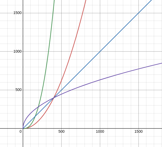
The power function for various values of m and n. Source: author, plotted on desmos.com
If we take the simplest curve, \( y = x \) which is the bonding curve for our token ABT (Alice-Bob token). Let us see how it affects user behaviour.
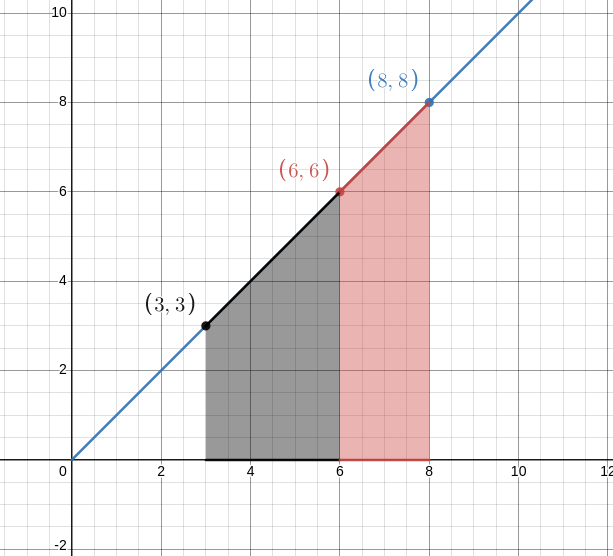
The area represents the price for the tokens at different supply levels. Source: author, plotted on desmos.com
If Alice buys token when the supply is low, she has to pay a small amount. She bought 3 tokens when the price was 3 ETH and now the tokens in supply is 6 tokens so the token price rises to 6 ETH. Bob notices that the token has increased in demand so he wants to have some of ABT too. He buys 2 ABT for 6 ETH each. Now, Alice can sell her stock of ABT as the token price is higher than her cost price and reap a profit out of it. Meanwhile, Bob would incur a loss if he sells after Alice has sold her stock since the token price is higher than his cost price. Thus, this curve incentivises users to buy early and rewards early adopters.
I should clarify that the statement “He buys 2 ABT for 6 ETH each” is not correct but a simplification. Since these are continuous curves, the price of assets are continuously changing, hence the price of ABT would increase for even a \( 10^{-18} \) part change. Thus, to compute the cost for 2 ABT, the contract would actually compute the area under curve for the function under appropriate limits. This can be done by good ‘ol integral calculus.
Let’s say that the number of tokens in circulation was t, and we want to buy k more tokens. By putting limits,
By solving for k, we can find the number of tokens that one can trade for p units of ETH or stablecoin, likewise:
The problem with the above formula is ofcourse the pesky exponent term which can lead to overflow for large t or n. How can we compute p and k efficiently. We need some math trickery and this is exactly what the bancor formulae are.
Bancor formula
If we define the initial pool balance that is the cost of going from 0 to t as another variable, say b, then the above expressions can be written as follows:
We still have to compute the exponent but we are getting there, bancor formula introduced another variable called the reserveRatio as follows:
Thus, the price formula under the bancor parameterisation becomes:
If you have had some prior exposure to basic economics then the above bonding curve seems a little disconcerting. Why is the price more when there are more tokens in circulation? Shouldn’t the price be more when the tokens are scarce? But think about it for a minute. More tokens in circulation means more demand. It is not like more tokens implies less scarcity.
Sigmoid functions as bonding functions
People coming from ML are already acquainted with the sigmoid function, a friendly little function with a nice shape.
However, the integral of this function is:
which is a hairy function to compute on the EVM as an infinite power series has to be summed. Smart contracts ideally cannot implement fancier curves as they cost more gas price to compute on-chain. But there is a similar function with a much nicer integral:
and, more importantly,
Now, just like m and n in the power bonding function, we can parameterise this function as follows and compute the sigmoid price function:
which when integrated within proper limits yield the following price function:
which is much easier to compute.
Price discovery mechanism
Quantitatively, the value of a token can be defined as the sum of total cash flow available to the bearer. But this raises many questions such as is it always possible to determine the future cash flow from an asset? If yes, then how to compute that? Traditional pricing techniques have evolved tools to price options and futures such as Black-Sholes formula, etc. but I haven’t researched much into that. The precise token design is also affected by the amount of token in circulation. Is it possible to value a token in the future if one allows infinite token minting by design? How to do that? These questions are under active research and no doubt, bonding curves will be an important part of future DeFi protocols.
Problems with bonding curves
Not a problem per se but I just wanted to note that AMMs are useful to provide liquidity to a token when it is in its infancy. But once the token is liquid enough to be traded on the free market at other DEXes, then who sets the price? Well, then the AMM and the free market stay at the same price. Any difference is levelled out by arbitrage.
- Frontrunning a transaction
Do you remember the case for ABT token above? Well, what if Eve got to know that Alice is about to buy her tokens, somehow places an exact transaction with a higher gas fee to incentivise miners to mine her transaction as oppose to Alice’s and then sell her tokens to Alice at a higher price (since the token’s price has just increased). One possible solution is limiting the gas fee that one can set for these transactions and always ask buyers/sellers to set it to that value.
- Nested bonding curves compounds risks
Imagine that ABT is pegged to ETH with a reserve ratio of 50%. Now, Darlene designs a token and pegs it to ABT with a reserve ratio of 10%. The actual reserve ratio is .5 * .1 = .05 or 5% of ETH. Further nesting can result in a highly volatile asset which basically means huge changes in the value of the asset for tiny changes in the value of the underlying asset (ETH in this case). One possible solution is to limit the number of nesting, of course.
REFERENCES
- How to make continuous bonding token models by Slava Balasanov.
- Bonding Curves in Depth: with math by Slava Balasanov.
- Token Curve Design by Parameters.
- Converting between bonding curve and bancor parameters by billy Rennekamp.
- Ethereum tokens explained by Linum Labs.
- Introduction to bonding curves, shapes, and use cases by Linum Labs.
Basil | @itbwtsh
Tech, Science, Design, Economics, Finance, and Books.
Basil blogs about complex topics in simple words.
This blog is his passion project.